Example 5: Plot a section along two points

This example demonstrates how to import file and draw a section plot along two points with GINCCO_lib using GINCCO_lib.heatmap_plot.plot_section() and GINCCO_lib.heatmap_plot.plot_section_contourf().

Code Example

Now we will import the library and the grid

# =========================
# IMPORTS
# =========================
import numpy as np
from netCDF4 import Dataset
from datetime import *
import GINCCO_lib as gc

# =========================
# CONFIGURATION
# =========================
tstart = datetime(2010, 1, 1)
tend   = datetime(2010, 10, 30)

path      = '/work/users/tungnd/GOT271/GOT_REF5/OFFLINE/'
file_name = '20130128_120000.symphonie.nc'

# =========================
# LOAD GRID AND DEPTH
# =========================
fgrid   = Dataset(path + 'grid.nc', 'r')
lat_t   = fgrid.variables['latitude_t'][:]
lon_t   = fgrid.variables['longitude_t'][:]
mask_t_var = fgrid.variables['mask_t']
if mask_t_var.ndim == 3:
    mask_t = mask_t_var[0, :, :]
elif mask_t_var.ndim == 2:
    mask_t = mask_t_var[:, :]

depth_t = fgrid.variables['depth_t'][:]

# Apply mask: set land values to NaN
if mask_t.shape == depth_t.shape:
    # Case 1: mask_t already 3D, same shape as depth_t
    depth_t[mask_t == 0] = np.nan
elif mask_t.ndim == 2 and depth_t.ndim == 3:
    # Case 2: mask_t is 2D, need to expand to match depth_t
    mask_3d = np.broadcast_to(mask_t, depth_t.shape)
    depth_t[mask_3d == 0] = np.nan
else:
    raise ValueError(f"Incompatible shapes: depth_t {depth_t.shape}, mask_t {mask_t.shape}")

Now select the section

# ============================================================
# EXAMPLE: Extract and plot a salinity section
# ============================================================

# Step 1: Define section endpoints
lon_p = [106, 107.5]
lat_p = [19, 18]

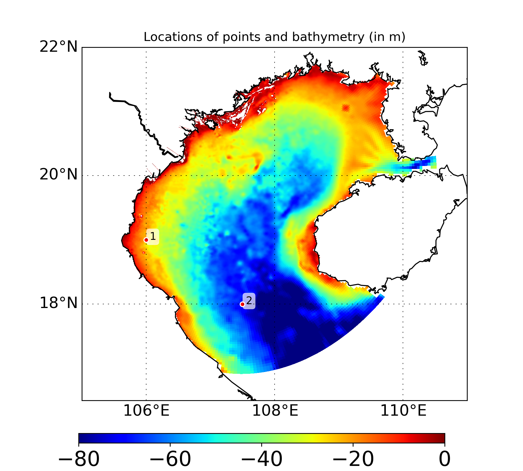
# Step 2: Plot section endpoints on bathymetry map
gc.map_draw_point(
    lon_min=105, lon_max=111,
    lat_min=16.5, lat_max=22,
    title="Locations of points and bathymetry (in m)",
    lon_data=lon_t,
    lat_data=lat_t,
    data_draw=depth_t[0, :, :],
    lat_point=lat_p,
    lon_point=lon_p,
    path_save="/prod/projects/data/tungnd/figure/",
    name_save="demo_7"
)

Now import data

# Step 3: Import section data
depth_out, data_out = gc.import_section(
    path=path,
    file_name=file_name,
    var='sal',
    lon_min=lon_p[0], lon_max=lon_p[1],
    lat_min=lat_p[0], lat_max=lat_p[1],
    M=80,
    depth_interval=0.5
)

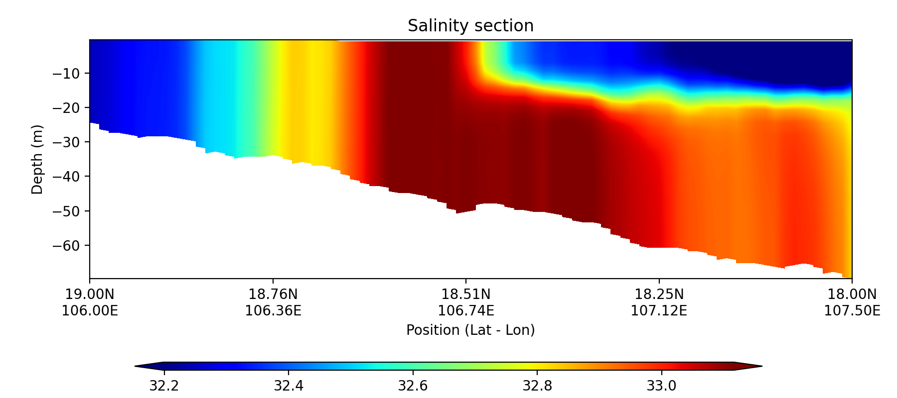
Plot using pcolormesh

# Step 4: Plot section heatmap
gc.plot_section(
    title='Salinity section',
    data_draw=data_out,
    depth_array=depth_out,     # ndarray, shape (depth, M)
    lon_min=lon_p[0], lon_max=lon_p[1],
    lat_min=lat_p[0], lat_max=lat_p[1],
    path_save="/prod/projects/data/tungnd/figure/",
    name_save="section",
    n_colors=100,   # number of discrete color bins
    n_ticks=5
)

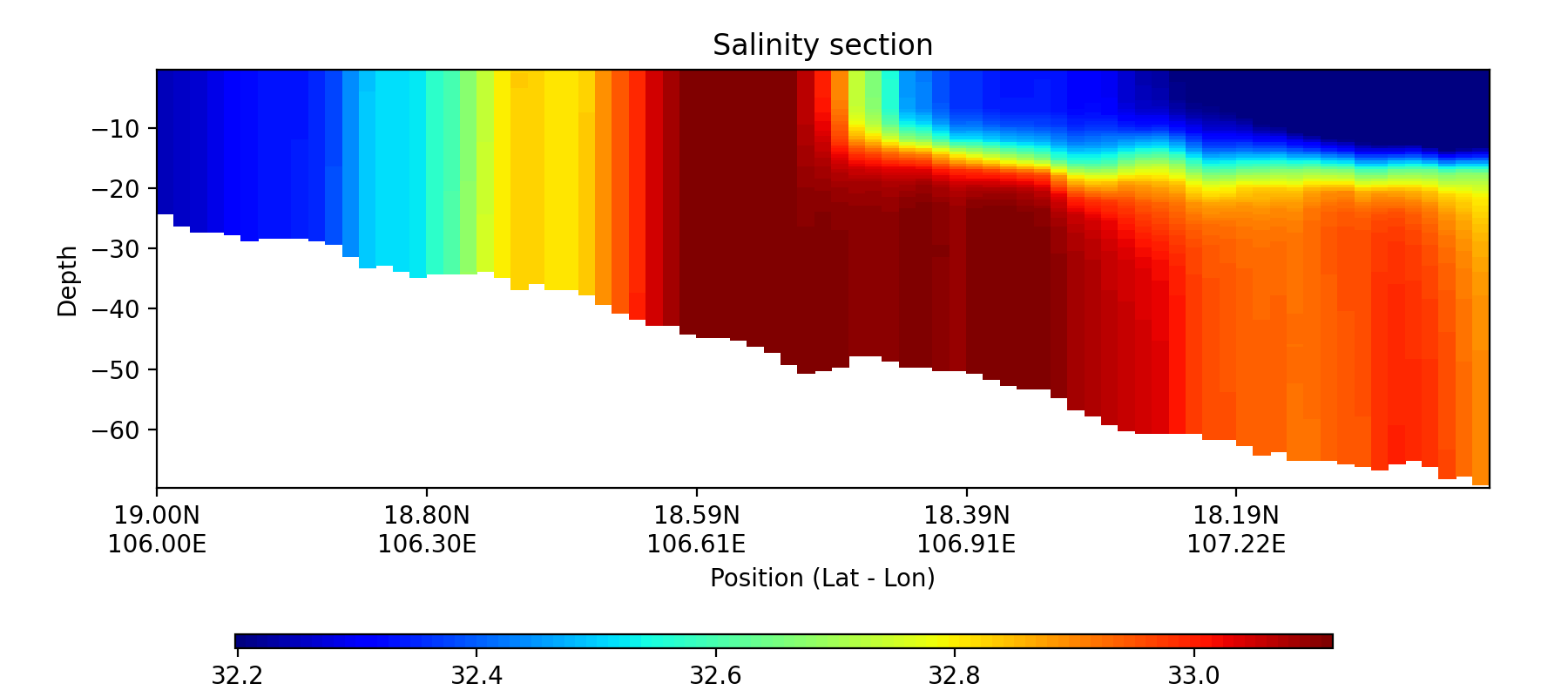
Plot using contourfill

# Step 4: Plot section heatmap
gc.plot_section_contourf(
    title='Salinity section',
    data_draw=data_out,
    depth_array=depth_out,     # ndarray, shape (depth, M)
    lon_min=lon_p[0], lon_max=lon_p[1],
    lat_min=lat_p[0], lat_max=lat_p[1],
    path_save="/prod/projects/data/tungnd/figure/",
    name_save="section",
    n_colors=250,   # number of discrete color bins
    n_ticks=5
)